🎨 Seeing precision change

This tutorial makes a picture of paths and precision from a real solve: where the adaptive-precision tracker decides double precision is no longer enough and raises its working precision. It builds directly on 👀 Watching paths: observers and path data (read that first for how observers and PathDataCollector work).

The idea

We solve cyclic-5 with the adaptive-precision Cauchy solver, with an attached SolutionPathCollector. That meta-observer attaches a fresh PathDataCollector to whichever tracker actually runs each path, and harvests the whole journey toward \(t \to 0\) (endgame included) into one pandas DataFrame per path. Each row is one accepted step, with the time, the space point, and the per-step diagnostics condition_number and precision.

# we are here to WATCH tracking: with ambient recording on, a repeated identical run
# would RECALL instead of tracking, and the observers would collect nothing to draw
pb.recording(False)


N = 5
ENDGAME_BOUNDARY = 0.1   # default t at which the endgame begins
HOMVAR_INDEX = 0         # homogenize() prepends the homogenizing coordinate


def cyclic_system(n):
    """The cyclic-n system (same construction as examples/solve_cyclic.py)."""
    x = [pb.Variable('x{}'.format(i)) for i in range(n)]
    w = x + x
    sys = pb.System()
    for length in range(1, n):
        sys.add_function(np.sum([np.prod(w[start:start + length]) for start in range(n)]))
    sys.add_function(np.prod(x) - 1)
    sys.add_variable_group(pb.VariableGroup(x))
    return sys


def collect_paths():
    """Solve cyclic-5 with AMP+Cauchy, capturing every solution path via an observer.

    Uses the purpose-built SolutionPathCollector: attached to the SOLVER, it grabs the tracker that
    actually runs each path (clone-safe under threading) and collects the whole journey to t -> 0,
    endgame included -- one PathDataCollector per solution path.  Returns a list of per-path
    DataFrames.
    """
    pb.random.set_random_seed(1)   # deterministic homotopy
    solver = pb.ZeroDimSolver(cyclic_system(N), endgame='cauchy', mptype='adaptive', startsystem='binomial')

    collector = pb.SolutionPathCollector()
    solver.add_observer(collector)
    solver.solve()

    return [s.as_dataframe() for s in collector.series if len(s) > 0]

Each path’s DataFrame carries everything the picture needs:

>>> paths = collect_paths()
>>> paths[0].columns.tolist()
['t', 'z0', 'z1', 'z2', 'z3', 'z4', 'z5', 'abs_t', 'condition_number', 'precision', 'stepsize']

Plotting

We plot, for every path:

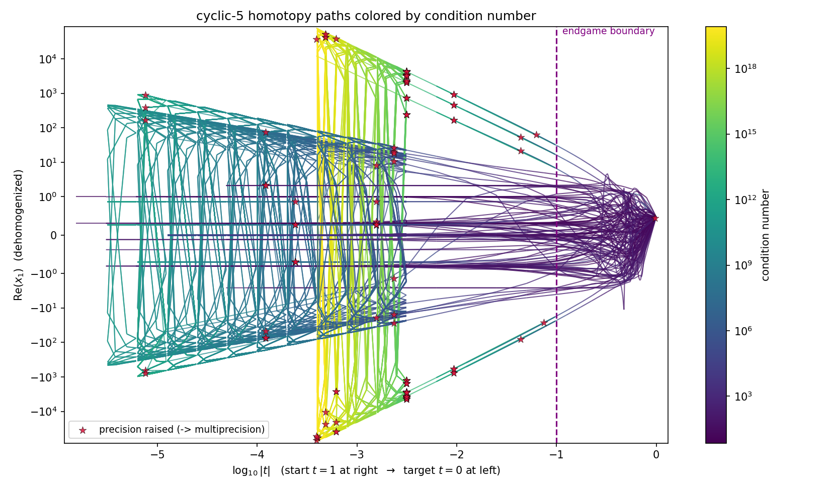
• x = \(\log_{10}|t|\), so the start (\(t=1\)) is on the right and the target (\(t \to 0\)) is on the left — logarithmic time, because all the interesting structure is near \(t=0\), and the endgames track toward the end time on a geometric series of timepoints;

• height = the real part of a dehomogenized coordinate. Paths weave and fan out to the distinct endpoints; a path going to infinity has its homogenizing coordinate go to zero, so the dehomogenized height shoots off

• color = the condition number along the path (log scale);

• a vertical line at the endgame boundary (\(t = 0.1\));

• a star wherever the tracker raised its working precision.

The full plotting routine is in the example script; the heart of it is coloring each path by its condition number with a LineCollection and scattering a marker at each precision increase:

        pts = np.array([x, y]).T.reshape(-1, 1, 2)
        segs = np.concatenate([pts[:-1], pts[1:]], axis=1)
        lc = LineCollection(segs, cmap=cmap, norm=norm, linewidths=1.0, alpha=0.75)
        lc.set_array(np.clip(cond[:-1], norm.vmin, norm.vmax))
        ax.add_collection(lc)

        inc = np.where(np.diff(prec) > 0)[0] + 1   # indices where precision rose
        esc_x.extend(x[inc]); esc_y.extend(y[inc])

Run the whole thing (needs matplotlib and pandas):

python python/docs/source/tutorials/seeing_precision_change/amp_precision_plot.py

Reading the picture

• On the right (near \(t=1\)) the paths emerge from a tight cluster of start points (in this projection) and are uniformly dark: low condition number, double precision. Pre-endgame tracking is easy.

• Color rises (toward yellow) as paths approach \(t=0\), and the precision-raise stars appear almost entirely to the left of the endgame boundary. Precision tracks conditioning, and the hard conditioning lives in the endgame.

• The paths that diverge to infinity (homogenizing coordinate \(\to 0\)) are the highest-condition ones (bright) and shoot to the top/bottom of the height axis; they legitimately need multiprecision before the solver truncates them. This is why it is a good idea to truncate infinite paths (though, silviana notes this is in practice a hard problem, to know what infinity actually is)

• The finite, well-conditioned paths — the ones whose endpoints are the actual cyclic-5 solutions — stay dark and starless essentially all the way in.

Note

That last point is the payoff of a specific bugfix. Before this, the cost model fed a predictor error-proportionality constant (size_proportion, which blows up to ~\(10^{51}\) in the endgame roundoff regime) into AMP Criterion B as if it were the latest Newton residual, and forced 39 of the 70 finite paths into multiprecision even though all 70 converge in pure double. With Criterion B reading the actual Newton residual instead, almost every finite path now stays in double — visible here as the near-absence of stars on the well-conditioned paths. The same observer machinery that drew this picture is exactly how that diagnosis was made: attach, collect, look.