🔁 Parameter homotopy

Todo

This is not a good example because the parameter homotopy saves 0 paths…

Todo

the homotopy is the “cheater’s homotopy” not a coefficient parameter homotopy. Rewrite this so the homotopy is just in the coefficients.

The most expensive part of homotopy continuation is the first solve – the one that has to find every solution from scratch. But a great many problems are really a family of systems that differ only in their coefficients: the same equations, evaluated at different parameter values. The eigenvalues of \(A(s)\) as \(s\) varies; the intersections of a fixed curve with a moving line; a design swept across a range of settings.

For such a family you should solve once, at generic complex parameter values, and then reuse those solutions as the start points of a parameter homotopy that deforms the coefficients to whatever value you actually care about – as many times as you like, each move tracking just the solutions you already have.

The tools are bertini.nag_algorithm.straight_line_homotopy() (builds the homotopy) and bertini.HomotopySolver() (runs the full zero-dim pipeline – pre-endgame tracking, the midpath check, the endgame, post-processing – from a homotopy you constructed and a list of start points you already have).

A family of systems

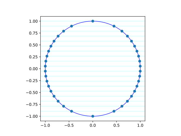
Take a fixed unit circle intersected with a horizontal line whose height is the parameter:

import bertini
from bertini import nag_algorithm

bertini.records_dir("circle_sweep_records")   # one line: record everything below
bertini.random.set_random_seed(42)            # same seed => reruns resume, not recompute

# the variables are SHARED across every member of the family: the parameter homotopy
# interpolates the members' equations, so they must be built over the same Variable objects.
x, y = bertini.Variable('x'), bertini.Variable('y')

def sys_instance(s):
    """The system { x^2 + y^2 - 1, 2y - s }: the unit circle meeting the line y = s/2."""
    sys = bertini.System()
    sys.add_variable_group(bertini.VariableGroup([x, y]))
    sys.add_function(x*x + y*y - 1)
    sys.add_function(2*y - s)
    return sys

Ab initio solve

Pick a generic complex member and solve it the usual way (a total-degree start system). Its two solutions are the start points we will reuse forever after:

start_param_val = bertini.random_complex()
generic = sys_instance(start_param_val)
first = bertini.ZeroDimSolver(generic, mptype='adaptive')
first.solve()
start_points = first.all_solutions()

Move the parameter

To reach another member, build the parameter homotopy from that member back to the generic one and track the start points through it:

target = sys_instance(0)                                 # the line y = 0
H = nag_algorithm.straight_line_homotopy(target, generic, gamma=1)
solver = bertini.HomotopySolver(H, start_points, target)
solver.solve()
# solver.all_solutions() are now (+/- 1, 0)

straight_line_homotopy(target, generic, gamma=1) is just \((1-t)\,\text{target} + t\,\text{generic}\) with t as the path variable: at \(t=1\) it is generic (so its solutions are our start points) and at \(t=0\) it is target.

Because we are making a homotopy in parameter space from generic to specific, we do not need the gamma trick, so gamma=1 is set when we construct the homotopy.

Now the payoff – sweep as many parameters as you want, reusing the same start points, never solving an expensive ab initio system from scratch again:

import numpy as np
results = {'param_vals':[], 'solns':[]}
for s in np.linspace(-2, 2, 20, dtype=bertini.real_mp):                               # lines y = 0, -1/2, 1/2
    target = sys_instance(s)
    H = nag_algorithm.straight_line_homotopy(target, generic, gamma=1)
    solver = bertini.HomotopySolver(H, start_points, target)
    solver.solve()
    roots = [p for p in solver.all_solutions()]
    for p in roots:
        xv, yv = complex(p[0]), complex(p[1])
        assert abs(xv*xv + yv*yv - 1) < 1e-8       # on the circle
        assert abs(2*yv - np.float64(s)) < 1e-8                # on the line y = s/2

    results['param_vals'].append(s)
    results['solns'].extend(solver.real_solutions())

Each iteration tracks only the two solutions we already have, to the new line – not a fresh total-degree solve. Across a large sweep that is the difference between tracking a handful of paths per parameter and tracking the full Bézout count every time.

A plot

I saved only the real solutions for each parameter point. Here they are plotted, together with the circle and the lines.

A note on the recording system in Bertini 2

The line of code back at the top

bertini.records_dir("circle_sweep_records")

were not decoration. Naming the ambient directory with records_dir turns recording on for every solver in the process – the bare ZeroDimSolver and HomotopySolver used here included, not just bertini.solve(). Every solve above wrote durable records of what it computed, and every solve consults the records before computing. The pinned seed is what makes that pay: with the same seed a rerun of the script rebuilds the same homotopies (randomness is seed-rooted), so every already-answered solve recalls from the records instead of tracking again. Kill a thousand-member sweep at member 700 and rerun – the first 700 come back nearly instantly and the sweep continues where it died. Without a pinned seed each run draws fresh randomness, and there is nothing to resume from.

Complete example

parameter_homotopy.py

"""Parameter homotopy: solve once, re-solve many times (Bertini 2 tutorial).

Fixed unit circle meeting a moving horizontal line y = s/2.
Run:  python parameter_homotopy.py
"""

import bertini
from bertini import nag_algorithm

bertini.records_dir("circle_sweep_records")
bertini.random.set_random_seed(42)

# the variables are SHARED across every member of the family: the parameter homotopy
# interpolates the members' equations, so they must be built over the same Variable objects.
x, y = bertini.Variable('x'), bertini.Variable('y')


def sys_instance(s):
    """The system { x^2 + y^2 - 1, 2y - s }: the unit circle meeting the line y = s/2."""
    sys = bertini.System()
    sys.add_variable_group(bertini.VariableGroup([x, y]))
    sys.add_function(x*x + y*y - 1)
    sys.add_function(2*y - s)
    return sys


def step_one():
    """Pick a generic member and solve it ab initio; its solutions are our start points."""
    start_param_val = bertini.random_complex()
    generic = sys_instance(start_param_val)
    first = bertini.ZeroDimSolver(generic, mptype='adaptive')
    first.solve()
    start_points = first.all_solutions()
    return generic, start_points


def sweep(generic, start_points):
    """Sweep many parameters, reusing the same start points, never solving from scratch."""
    import numpy as np
    results = {'param_vals':[], 'solns':[]}
    for s in np.linspace(-2, 2, 20, dtype=bertini.real_mp):                               # lines y = 0, -1/2, 1/2
        target = sys_instance(s)
        H = nag_algorithm.straight_line_homotopy(target, generic, gamma=1)
        solver = bertini.HomotopySolver(H, start_points, target)
        solver.solve()
        roots = [p for p in solver.all_solutions()]
        for p in roots:
            xv, yv = complex(p[0]), complex(p[1])
            assert abs(xv*xv + yv*yv - 1) < 1e-8       # on the circle
            assert abs(2*yv - np.float64(s)) < 1e-8                # on the line y = s/2

        results['param_vals'].append(s)
        results['solns'].extend(solver.real_solutions())

    # some converting to facilitate plotting
    results['param_vals'] = np.array(results['param_vals'], dtype=np.float64)
    results['solns'] = np.array(bertini.real(results['solns']), dtype=np.float64)
    return results


def plot(results):
    solns = results['solns']

    import matplotlib.pyplot as plt
    ax = plt.gca()

    line_x_min = -10
    line_x_max = 10

    for s in results['param_vals']:
        # 0 = 2*y - s
        # y = s/2 # a horizontal line at height s/2
        ax.plot([line_x_min, line_x_max], [s/2,s/2],color='xkcd:pale blue',zorder=1) # https://xkcd.com/color/rgb/

    circle = plt.Circle((0,0), 1, color='b', fill=False,zorder=2)


    ax.add_patch(circle)
    ax.scatter(solns[:,0],solns[:,1], zorder=3)
    ax.set_aspect('equal', 'box')
    ax.axis([-1.1, 1.1, -1.1, 1.1])

    plt.savefig('parameter_homotopy_circle.png')
    plt.savefig('parameter_homotopy_circle.svg')

def main():

    generic, start_points = step_one()
    results = sweep(generic, start_points)

    plot(results)


if __name__ == '__main__':
    main()