〰️ Tracking an analytic homotopy

The tracking nonsingular solutions tutorial pauses partway through to add a sine to a system, observes that its degree comes back as -1, remarks that homotopy continuation on non-algebraic systems is possible anyway, and then deletes the system and goes back to polynomials.

This page picks up where that other tutorial turned away.

Why there is no start system

A start system exists to be solved with little, and to have enough roots to reach every solution of the target. Both halves lean on the degree. A total-degree start system is built from the degrees of the target’s functions, and the number of paths it provides is their product.

Sine has no degree. Ask, and Bertini tells you so:

x = bertini.Variable('x')
sys = bertini.System()
sys.add_variable_group(bertini.VariableGroup([x]))
sys.add_function(bertini.symbolics.sin(x) - bertini.coefficient('1/2'))

print(sys.degrees())
print(sys.is_polynomial())

[-1]
False

That is not an evasion, it is the truth: \(\sin(x) = 1/2\) has infinitely many solutions, and no finite number of paths can reach them all. The refusal to make a start system says so out loud.

try:
    bertini.system.start_system.TotalDegreeLinearProduct(sys)
except RuntimeError as refused:
    print('refused')

refused

A homotopy with sine in it

Strictly speaking, path tracking doesn’t really need a start system. It actually just needs a homotopy and points to start from.

Let’s build the two ends of the homotopy as ordinary systems and glue them together. At \(t = 1\) the homotopy is gamma*sin(x), whose roots are the integer multiples of \(\pi\); at \(t = 0\) it is the target.

target = bertini.System()
target.add_variable_group(bertini.VariableGroup([x]))
target.add_function(bertini.symbolics.sin(x) - bertini.coefficient('1/2'))

start = bertini.System()
start.add_variable_group(bertini.VariableGroup([x]))
start.add_function(bertini.symbolics.sin(x))

gamma = bertini.coefficient('-24/25') + bertini.I * bertini.coefficient('7/25')
H = bertini.system.make_homotopy(target, start, gamma=gamma)

print(H.have_path_variable(), H.num_functions(), H.degrees())

True 1 [-1]

print(H) shows what was built:

1 variable group:
  group 0: x

1 function:
  f_0 = (sin(x)-1/2)*(1-t)+((0+1*I)*7/25+(-24/25))*t*sin(x)

path variable: t

The homotopy inherits the -1: a blend of functions is polynomial only when every part is.

That gamma is the exact rational point \((-24 + 7i)/25\) on the unit circle, from the Pythagorean triple 7-24-25. (A random gamma would do the same job; an exact one makes this page reproduce byte for byte for doctesting purposes.) Keeping coefficients exact matters more than usual here, because a decimal string becomes a binary float and any noise in a coefficient moves the singularity structure you are about to look at.

You choose the start points for analytic systems

Here is the part with no polynomial analogue. Nobody can hand you all the solutions, so you decide which ones you want by choosing where to start. Five multiples of \(\pi\) will chase five roots.

pi = bertini.multiprec.real_mp('3.14159265358979323846264338327950288419716939937511')
start_points = [np.array([bertini.multiprec.complex_mp(pi * k)]) for k in (-2, -1, 0, 1, 2)]

Want more roots? Start from more multiples.

Fixed multiple precision tracking

solver = bertini.HomotopySolver(H, start_points, target, mptype='multiple')
solver.solve()

ends = sorted(round(complex(s[0]).real, 9) for s in solver.all_solutions())
print(ends)

[-5.759586532, -3.665191429, 0.523598776, 2.617993878, 6.806784083]

Every one of those is a root of \(\sin x = 1/2\), which the closed form puts at \(\arcsin(1/2) + 2\pi k\) and \(\pi - \arcsin(1/2) + 2\pi k\). Checking against it:

exact = [np.arcsin(0.5) + 2 * np.pi * k for k in (-1, 0, 1)] + \
        [np.pi - np.arcsin(0.5) + 2 * np.pi * k for k in (-1, 0, 1)]
worst = max(min(abs(e - w) for w in exact) for e in ends)
print(worst < 1e-9)

True

Five starts, five distinct roots, each correct to the tolerance we asked for.

Adaptive precision needs you to provide some bounds

mptype='multiple' above was not an accident. Ask for the default, adaptive precision, and Bertini declines:

try:
    bertini.HomotopySolver(H, start_points, target, mptype='adaptive')
except ValueError as refused:
    print(str(refused).split('.')[0])

HomotopySolver: this homotopy is not polynomial, and adaptive precision needs a degree bound it therefore cannot have

Adaptive precision decides how many digits a step needs by comparing measured quantities against two error bounds, one for evaluating the functions and one for evaluating the Jacobian. For a polynomial system, those bounds come from its degree and the size of its coefficients. With no degree there is no such recipe, and the criteria have nothing to compare against.

Fixed precision carries no such constants, which is why it just works. Choose enough digits for the problem and the tracker does the rest.

If you want adaptive precision, you supply the two bounds yourself, and the solver takes them:

config = bertini.tracking.AMPConfig()
config.jacobian_eval_error_bound = 8
config.function_eval_error_bound = 4
config.linear_solve_error_bound = 1

adaptive = bertini.HomotopySolver(H, start_points, target,
                                  mptype='adaptive', amp_config=config)
adaptive.solve()
print(len(adaptive.all_solutions()))

5

Numbers you can defend for your own system, that is. What those bounds should be for an analytic system feels like a genuinely open question, and a reading is gathered in issue 439.

Endgames work correctly for analytic systems

Push the right-hand side from 1/2 to 1 and the roots collide: \(\sin x = 1\) has a double root at \(\pi/2\). This is where you might expect the machinery to give up, since the endgame’s theory is usually stated for polynomials. But check this out:

target = bertini.System()
target.add_variable_group(bertini.VariableGroup([x]))
target.add_function(bertini.symbolics.sin(x) - bertini.coefficient(1))

H = bertini.system.make_homotopy(target, start, gamma=gamma)
start_pts = [np.array([bertini.multiprec.complex_mp(pi * k)]) for k in (0, 1)]

solver = bertini.HomotopySolver(H, start_pts, target, mptype='multiple')
solver.solve()

print([m.cycle_num for m in solver.solution_metadata()])
print([round(complex(s[0]).real, 6) for s in solver.all_solutions()])

[2, 2]
[1.570796, 1.570796]

Cycle number 2, correctly, and both paths land on \(\pi/2\).

It works for a reason worth knowing. The power series endgame assumes the path behaves like a Puiseux series near its endpoint, which is a statement about algebraic branching. The Weierstrass Preparation Theorem says that an analytic function with an isolated zero of order \(k\) factors locally as a unit times a polynomial of degree \(k\). Near a finite endpoint, an analytic family branches exactly like an algebraic one, and the endgame’s assumption survives. The endgames are super cool in another way, too: nothing in the cycle-number estimation routine consults a system’s degree.

Two pictures

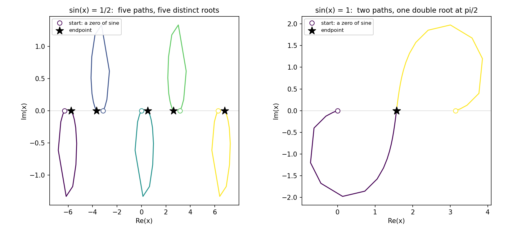
Analytic paths in the complex plane. Open circles are the roots of sine we chose to start from, stars are the endpoints, and each vertex is a step the tracker took. Remember, the homotopy uses a complex gamma. On the left, five paths leave the real axis, loop through the complex plane and return to five distinct roots. On the right, the two paths approach \(\pi/2\) from opposite sides and arrive together.

Limits on analytic systems in Bertini 2

Worth being plain about the limits, since they are real and they are not bugs.

There is no solution count. No Bezout number bounds an analytic system, so “all solutions” is not a question this machinery answers. You get the endpoints of the paths you started.

There is no completeness guarantee. Choosing more start points finds more roots, and nothing tells you when to stop.

Paths that run to infinity have no theory behind them here. For a polynomial system, divergence is understood through the degree and projective space. But an exponential, for example, has an essential singularity at infinity, and the usual reasoning does not transfer. Tracking such a path is not forbidden; just do not expect the diverging-path heuristics to mean what they mean for a polynomial.

Lastly, adaptive precision needs bounds you chose, as above.

The source

tracking_analytic.py

# This file is part of Bertini 2.
#
# tracking_analytic.py is free software: you can redistribute it and/or modify
# it under the terms of the GNU General Public License as published by
# the Free Software Foundation, either version 3 of the License, or
# (at your option) any later version.
#
# tracking_analytic.py is distributed in the hope that it will be useful,
# but WITHOUT ANY WARRANTY; without even the implied warranty of
# MERCHANTABILITY or FITNESS FOR A PARTICULAR PURPOSE.  See the
# GNU General Public License for more details.
#
# You should have received a copy of the GNU General Public License
# along with tracking_analytic.py.  If not, see <http://www.gnu.org/licenses/>.
#
#  Copyright(C) Bertini2 Development Team
#
#  See <http://www.gnu.org/licenses/> for a copy of the license,
#  as well as COPYING.  Bertini2 is provided with permitted
#  additional terms in the b2/licenses/ directory.

"""The tutorial's runnable source, and the regenerator for its figure.

Tracks a homotopy whose functions are not polynomials -- sine -- and draws the paths in the
complex plane.  Two frames, side by side: five paths landing on distinct roots of
``sin(x) = 1/2``, and two paths colliding at a branch point of ``sin(x) = 1``.

Nothing here is random.  gamma is the exact rational point ``(-24 + 7i)/25`` on the unit
circle, and the start points are exact, so the picture is the same every time.

Run:  python tracking_analytic.py
      (or via tools/refresh_doc_artifacts.py --plots --only tracking_analytic)
"""

import matplotlib
matplotlib.use('Agg')            # headless: no display needed
import matplotlib.pyplot as plt

import numpy as np

import bertini
from bertini import SolutionPathCollector

PI_50 = '3.14159265358979323846264338327950288419716939937511'


def sine_homotopy(right_hand_side):
    """H = (1-t)*(sin(x) - c) + gamma*t*sin(x), and the target system it ends at.

    At t = 1 the homotopy is gamma*sin(x), whose roots are the integer multiples of pi.  At
    t = 0 it is the target, sin(x) = c.
    """
    x = bertini.Variable('x')

    target = bertini.System()
    target.add_variable_group(bertini.VariableGroup([x]))
    target.add_function(bertini.symbolics.sin(x) - bertini.coefficient(right_hand_side))

    start = bertini.System()
    start.add_variable_group(bertini.VariableGroup([x]))
    start.add_function(bertini.symbolics.sin(x))

    gamma = bertini.coefficient('-24/25') + bertini.I * bertini.coefficient('7/25')
    return bertini.system.make_homotopy(target, start, gamma=gamma), target


def zeros_of_sine(multiples):
    """Start points: the roots of sin(x) = 0 you choose to chase, as k*pi."""
    points = []
    for k in multiples:
        value = bertini.multiprec.real_mp(PI_50) * k
        points.append(np.array([bertini.multiprec.complex_mp(value)]))
    return points


def track(right_hand_side, multiples, mptype='multiple'):
    """Track the chosen start points, collecting every path.  Returns (solver, collector)."""
    homotopy, target = sine_homotopy(right_hand_side)
    solver = bertini.HomotopySolver(homotopy, zeros_of_sine(multiples), target, mptype=mptype)

    collector = SolutionPathCollector()
    solver.add_observer(collector)
    solver.solve()
    return solver, collector


def _affine(points):
    """The affine x-coordinate of a recorded path.  These systems are never homogenized, so the
    recorded points are already affine; the check keeps the helper honest if that changes."""
    return points[:, 0] if points.shape[1] == 1 else points[:, 1] / points[:, 0]


def _draw(ax, collector, solver, title):
    cmap = plt.get_cmap('viridis')
    series = collector.series
    for index, path in enumerate(series):
        x_of_t = _affine(path.points())
        color = cmap(index / max(len(series) - 1, 1))
        ax.plot(x_of_t.real, x_of_t.imag, '-', color=color, lw=1.4)
        ax.plot(x_of_t.real[0], x_of_t.imag[0], 'o', color=color, ms=7, mfc='white', zorder=4,
                label='start: a zero of sine' if index == 0 else None)

    ends = [complex(s[0]) for s in solver.all_solutions() if len(s)]
    ax.scatter([e.real for e in ends], [e.imag for e in ends],
               c='k', marker='*', s=150, zorder=5, label='endpoint')

    ax.axhline(0, color='0.85', lw=0.8, zorder=0)     # the real axis, where both ends live
    ax.set_title(title, fontsize=11)
    ax.set_xlabel('Re(x)')
    ax.set_ylabel('Im(x)')
    ax.legend(loc='upper left', fontsize=8, framealpha=0.9)


def plot():
    """Draw both frames and write the figure beside this file."""
    spread_solver, spread_paths = track('1/2', (-2, -1, 0, 1, 2))
    collide_solver, collide_paths = track(1, (0, 1))

    fig, axes = plt.subplots(1, 2, figsize=(11, 5))

    _draw(axes[0], spread_paths, spread_solver,
          'sin(x) = 1/2:  five paths, five distinct roots')
    _draw(axes[1], collide_paths, collide_solver,
          'sin(x) = 1:  two paths, one double root at pi/2')

    for ax in axes:
        ax.set_box_aspect(1)

    fig.tight_layout()
    fig.savefig('tracking_analytic.svg')
    fig.savefig('tracking_analytic.png', dpi=150)
    print('wrote tracking_analytic.svg and .png')


def report():
    """Print what the tutorial asserts, for anyone running this file directly."""
    solver, _ = track('1/2', (-2, -1, 0, 1, 2))
    ends = sorted(complex(s[0]).real for s in solver.all_solutions() if len(s))
    print('sin(x) = 1/2 endpoints:', [round(e, 12) for e in ends])
    print('arcsin(1/2)           :', round(float(np.arcsin(0.5)), 12))

    solver, _ = track(1, (0, 1))
    print('sin(x) = 1 cycle numbers:', [m.cycle_num for m in solver.solution_metadata()])
    print('pi/2                    :', round(float(np.pi / 2), 12))


if __name__ == '__main__':
    bertini.recording(False)          # a doc figure is not a run worth archiving
    bertini.default_precision(60)
    report()
    plot()