⏱️ Timing Bertini 1 vs Bertini 2

Bertini 2 is a from-scratch C++17 rewrite; a fair question is how its speed compares to Bertini 1.7. This tutorial benchmarks the two on the same systems and ends in a plot — and records what was timed and where, so the numbers can be refreshed as the library improves.

Comparing fairly

The fair way to compare two solvers is to hand them the same problem with the same settings. We build each system once in pybertini and emit it as a Bertini-1 classic input with System.to_classic_input(), which writes the equations and the tracking knobs (precision mode, predictor, tolerances, step cadence). Both solvers read that one file, each builds its own random start system, and solves. We time only the solver subprocess (never parsing/IO) and keep the fastest of a few repeats, serial (OMP_NUM_THREADS=1):

def time_solver(exe, input_text, repeats=3, timeout=600):
    """Fastest serial wall time (seconds) over `repeats` runs of `exe` on `input_text`; (time, count)."""
    best, count = float("inf"), None
    for _ in range(repeats):
        d = tempfile.mkdtemp()
        try:
            open(os.path.join(d, "input"), "w").write(input_text)
            env = dict(os.environ, OMP_NUM_THREADS="1")
            t0 = time.perf_counter()
            r = subprocess.run([os.path.abspath(exe), "input"], cwd=d, env=env,
                               stdout=subprocess.DEVNULL, stderr=subprocess.DEVNULL, timeout=timeout)
            dt = time.perf_counter() - t0
            if r.returncode == 0:
                best = min(best, dt)
                count = solution_count(d)
        finally:
            shutil.rmtree(d, ignore_errors=True)
    return (best if best < float("inf") else None), count

(The maintained, fuller harness — which also sweeps MPI ranks and appends a committed history.csv — is benchmark/comparison/run_comparison.py; this tutorial is a small self-contained cousin.)

Record the provenance

Timing numbers are meaningless without context, and they go stale. We capture the date, both solver versions (with the Bertini 2 git commit), and the machine, and stamp them onto the figure:

def provenance(b2_exe, b1_exe):
    """Record WHAT was timed and WHERE, so the numbers can be refreshed and stay interpretable."""
    here = os.path.dirname(os.path.abspath(__file__))
    try:
        commit = subprocess.run(["git", "-C", here, "rev-parse", "--short", "HEAD"],
                                capture_output=True, text=True).stdout.strip()
    except Exception:
        commit = ""
    cpu = platform.processor() or "unknown"
    try:
        if platform.system() == "Darwin":
            cpu = subprocess.run(["sysctl", "-n", "machdep.cpu.brand_string"],
                                 capture_output=True, text=True).stdout.strip() or cpu
    except Exception:
        pass
    b2 = _first_nonempty_version_line(b2_exe) + (" @ " + commit if commit else "")
    return {"date": datetime.date.today().isoformat(),
            "b2": b2,
            "b1": _first_nonempty_version_line(b1_exe),
            "machine": "{} / {} {}".format(cpu, platform.system(), platform.release())}

The result

Run it (needs matplotlib; Bertini 1 optional):

python python/docs/source/tutorials/bertini1_vs_bertini2_timing/b1_vs_b2_timing.py \
    --bertini2 ./build/core/bertini2 --bertini1 /usr/local/bin/bertini --out .

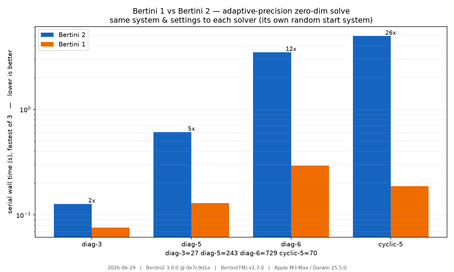
How to read it (for the run shown — see the caption for date/versions/machine):

• Bertini 2 is still slower than Bertini 1 on these problems — from a small factor on the tiny diagonal system to ~25× on cyclic-5. This is honest: Bertini 1 is hand-tuned C with its own linear algebra; Bertini 2 trades constant-factor speed for a templated, observable, arbitrary-precision design.

• The diagonal family diag-3/5/6 is well-conditioned (every path stays in double precision), so its growing slowdown is pure per-step tracking overhead scaling with problem size — a standing performance lever, independent of the endgame.

• cyclic-5 exercises the endgame. The adaptive-numeric-type endgame (the Cauchy and PowerSeries endgames now compute in hardware complex_dbl while a path’s conditioning allows, escalating to mpfr only when the tracker’s authority demands it) cut the endgame’s per-operation cost by roughly 10×. Where a path’s endgame stays in double — e.g. the default TotalDegreeBinomial start system — cyclic-5 in adaptive precision is now ~Bertini-1 speed (~0.4 s serial, with 0 of 70 finite paths needing to escalate above double).

  The bar shown here is larger than that, because this benchmark hands both solvers a total-degree classic input, and that start system currently makes Bertini 2’s endgame stall near \(t = 0\) (it takes far too many tiny steps). The run stays mostly in double — so the per-step speedup does apply — but the step count is the problem. That stall, not precision and not the endgame’s arithmetic, is the current top lever for this particular path, and is tracked separately from this endgame work.

Both solvers report the same solution counts (shown under the bars), so this is a like-for-like comparison, not a speed/accuracy trade.