🖼️ The classic continuation cartoon, from real data
Every introduction to homotopy continuation draws the same picture: smooth start points at \(t=1\) on the right, paths flowing left to the target’s solutions at \(t=0\), past an endgame boundary; the endpoints come in three flavors — nonsingular, singular, and “at infinity” (paths that diverge). Here is the hand-drawn version:
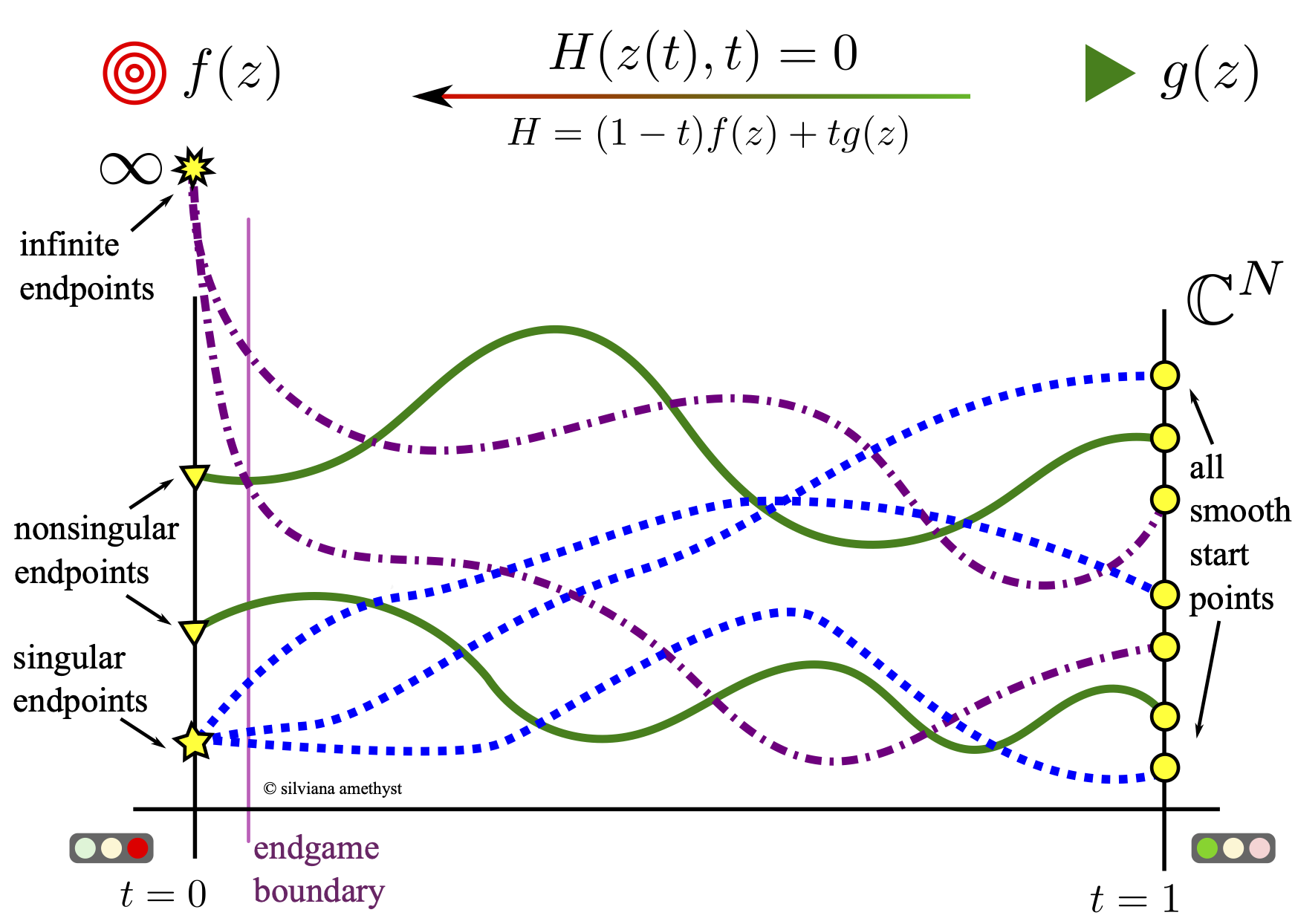
This tutorial reproduces that drawing from a real solve — every curve is genuine tracked data — with each path styled by the kind of endpoint it reaches. It builds on the observer machinery from 👀 Watching the paths: observers and path data.
A small system with one of each flavor
We want only a handful of paths, with a singular endpoint, a few nonsingular ones, and some that diverge. This system delivers exactly that:
Substituting \(y = x^2\) gives \((x-1)^2 (x+2)(x-4) = 0\): a double root at \(x=1\) — a singular endpoint reached by two paths — and simple roots at \(x=-2, 4\) (nonsingular). The total-degree start system has 6 paths, so the remaining two diverge to infinity (the homogenizing coordinate goes to zero).
Collecting the paths, classified by endpoint
Attach a SolutionPathCollector to the solver; it captures each path (the whole journey to
\(t \to 0\)). After solving, the per-path solution_metadata() tells us each endpoint’s
flavor, so we can style each curve:
def classify(meta):
    if not meta.is_finite:
        return "infinite"
    return "singular" if meta.is_singular else "nonsingular"


def collect():
    """Solve and return [(flavor, DataFrame), ...], one per path."""
    pb.random.set_random_seed(1)
    zd = ZeroDimSolver(target_system(), mptype="adaptive")
    coll = nobs.SolutionPathCollector()
    zd.add_observer(coll)
    zd.solve()
    md = zd.solution_metadata()
    out = []
    for series in coll.series:
        if len(series) == 0:
            continue
        out.append((classify(md[series.path_index]), series.as_dataframe()))
    return out
Note
The collector records the start point too, not just the accepted steps. Its
PathDataCollector watches TrackingStarted (which fires at \(t=1\), before any step)
in addition to SuccessfulStep — so every path begins at its start-system root on the right,
exactly as the cartoon shows. A step-only collector would start one step in, near
\(t \approx 0.9\).
Drawing it
A few choices turn the data into the cartoon:
height is a fixed generic complex projection of the dehomogenized coordinates down to one real number. A single coordinate’s real part would make the structured total-degree start points (scaled roots of unity) land on top of each other; a generic projection separates them.
the vertical axis is given a finite window sized to the finite roots, so the two paths that diverge to infinity do not compress everything else into a flat line. Each diverging path is drawn only up to where it leaves the window, then cut off with an \(\infty\) just inside the axis (no endpoint marker) — the cartoon’s “burst”.
each flavor gets a distinct line style and color and endpoint marker (so it survives grayscale / color-blind viewing): nonsingular solid
▽, singular dashed★, infinite dash-dot.a bullseye marks the target \(f(z)=0\) at \(t=0\), the start points (gold) sit on the right at \(t=1\), and the endgame boundary is drawn at \(t=0.1\).
Run it (needs matplotlib):
python python/docs/source/tutorials/classic_continuation_cartoon/classic_continuation_cartoon.py .
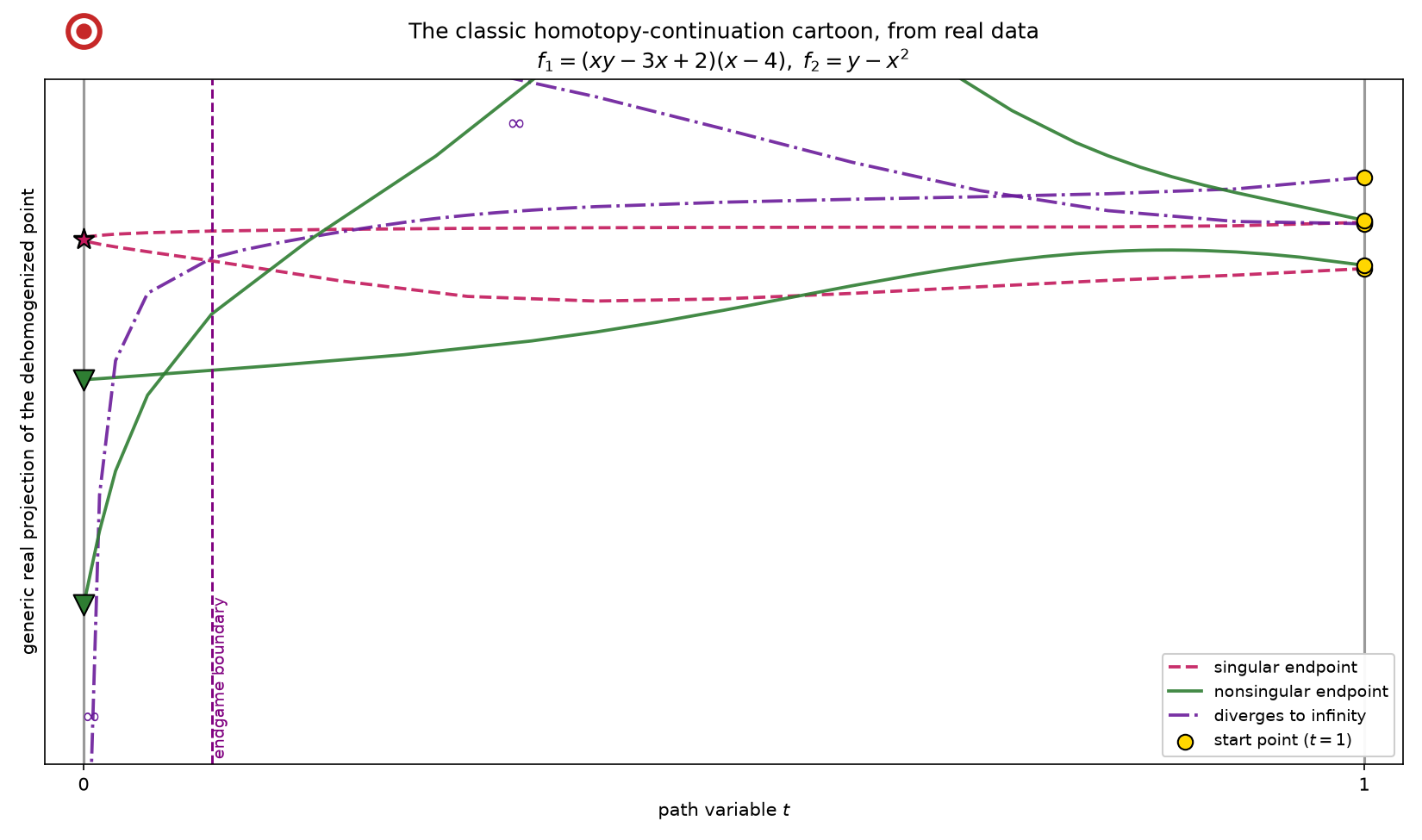
The same shape as the hand drawing — start points on the right, three flavors of endpoint on the left, two paths funnelling into the single singular point, two diverging to infinity — but now every wiggle is a real tracked path of an actual homotopy.
Note
The total-degree start points being scaled roots of unity (a structured set, not generic) is
exactly why a naive single-coordinate height collapses them. That structure is a known wart in
the current TotalDegreeLinearProduct start system; a genuinely randomized (linear-product) total-degree
start would put them in general position.