🧬 The Monodromy Loom

Take a polynomial whose coefficients depend on a parameter, and walk that parameter slowly around a closed loop. The roots move as it moves — and when the loop encircles the places where two roots collide, the roots come back permuted. That permutation is the family’s monodromy: its Galois action, made visible as a literal braid of tracked solution paths.

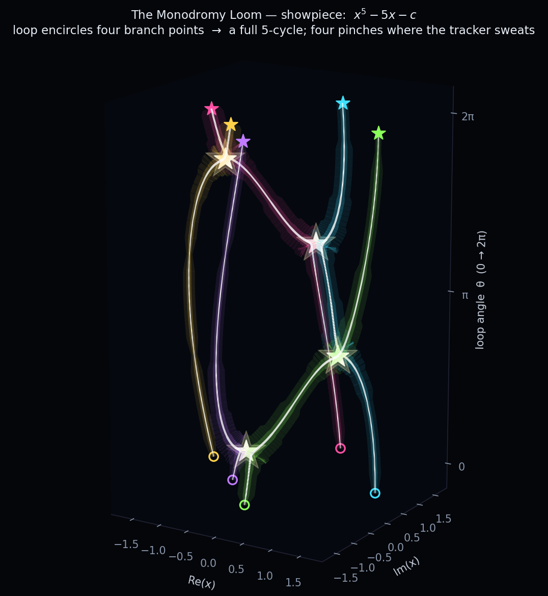
Every strand above is one root of \(f(x;c) = x^5 - 5x - c\), plotted in 3-D as \((\operatorname{Re} x,\ \operatorname{Im} x,\ \theta)\) where \(\theta\) is the loop angle running \(0 \to 2\pi\). As \(c\) circles once around all four branch points, the five roots weave through one another and land in a single 5-cycle — the generator of the family’s Galois group. The four white star-bursts are the near-collisions: each is where the loop grazes a branch point and a different pair of strands very nearly touches.

The texture is the tracker’s heartbeat

The strands are not uniform ribbons. Their brightness and width are the adaptive-precision tracker’s own diagnostics, streamed step-by-step from a PathDataCollector. Right at a pinch the Jacobian is nearly singular, so the tracker’s step size collapses and it piles up tiny steps to inch past — and exactly there the strand flares and swells. You are watching the solver work hardest precisely where the mathematics is hardest.

Start simple: one loop, one swap

Before the five-strand braid, the whole idea fits in a cubic. \(f(x;c) = x^3 - 3x - c\) has two branch points, at \(c = \pm 2\). Loop one of them and exactly two roots swap — a single transposition — while the third rides straight through, untouched:

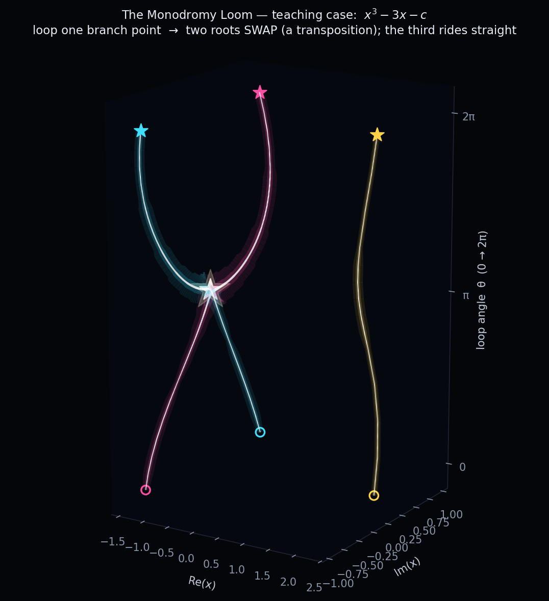
The two swapping strands (magenta and gold) cross at the glowing branch point at \(\theta=\pi\) — note how they brighten and thicken there as the tracker fights the near-collision — and their start rings at the base map to each other’s end stars at the top. The calm strand keeps its place. That is monodromy in one picture; the quintic is the same lesson, louder.

How it is built

The trick is to bake the entire loop into a single homotopy by making the coefficient a function of the path variable, \(c(t) = \text{center} + \text{radius}\cdot e^{\,i(\theta + \varphi)}\) with \(\theta = 2\pi(1-t)\). Then one continuous track per strand — from \(t=1\) (the start configuration) to \(t=0\) (the loop closed) — traces the whole loop, and the path variable maps straight onto the loop angle:

def loom_homotopy(degree, center, radius, phi_over_pi):
    """H(x, t) = x^d - d*x - c(t),  c(t) = center + radius*exp(i*(theta + phi)),
    theta = 2pi(1-t),  phi = phi_over_pi * pi.

    At t=1 theta=phi (the start configuration); at t=0 the loop has closed.  Tracking a root of the
    start configuration from t=1 to t=0 carries it once around the loop.
    """
    x = bertini.Variable('x')
    t = bertini.Variable('t')
    theta = 2 * bertini.Pi * (1 - t) + bertini.coefficient(phi_over_pi) * bertini.Pi
    sys = bertini.System()
    sys.add_function(x**degree - degree * x - _c_of_theta(theta, center, radius))
    sys.add_path_variable(t)
    sys.add_variable_group(bertini.VariableGroup([x]))
    return sys

Tracking every strand and capturing its trajectory is then just an AMPTracker with a PathDataCollector attached, once per root:

def track_loop(degree, center, radius, phi_over_pi, tol=1e-10):
    """Track every strand once around the loop.  Returns a list of per-strand dicts with the loop
    angle ``theta``, the complex position ``x``, and the tracker diagnostics along the path."""
    H = loom_homotopy(degree, center, radius, phi_over_pi)
    roots = start_configuration(degree, center, radius, phi_over_pi)

    tracker = bertini.AMPTracker(H)
    tracker.setup(bertini.tracking.Predictor.RK4, tol, 1e6,
                  tracking.SteppingConfig(), tracking.NewtonConfig())
    tracker.precision_setup(tracking.amp_config_from(H))

    strands = []
    for r in roots:
        collector = amp_observers.PathDataCollector()
        tracker.add_observer(collector)
        end = np.zeros(H.num_variables(), dtype=complex_mp)
        tracker.track_path(end, complex_mp(1.0, 0.0), complex_mp(0.0, 0.0),
                           np.array([complex_mp(r.real, r.imag)]))
        tracker.remove_observer(collector)

        times = collector.times()               # complex path-variable value per step
        pts = collector.points()[:, 0]           # affine x (one variable)
        dgn = collector.diagnostics()            # (n, 4): |t|, condition, precision, stepsize
        strands.append(dict(start=r, end=complex(end[0]),
                            theta=2 * math.pi * (1 - times.real), x=pts,
                            precision=dgn[:, 2], stepsize=dgn[:, 3]))
    return strands, roots

The rest — resampling the strands, colouring by step-size stress, and finding the pinches — is plotting; see monodromy_loom.py in full.

Why it matters

The braid is not decoration: it is the monodromy representation of the family. Reading the permutation off the strands recovers the Galois group of \(f(x;c)\) over \(\mathbb{C}(c)\), and the same loop-tracking is the engine behind monodromy methods in numerical algebraic geometry (decomposing solution sets, certifying trace tests). What makes it a showpiece here is that the picture carries three stories at once — the algebra (the braid), the geometry (the branch points the strands must wind around), and the numerics (the adaptive tracker sweating at every collision).

Note

This is a raster showpiece: PNG only (a 3-D render has no meaningful SVG), regenerated through tools/refresh_doc_artifacts.py. It is not a doctest — the code above is shown from the real generator, which you can also run directly with python monodromy_loom.py.