📍 A real point on every component (the Trott curve)¶

Homotopy continuation finds all the complex solutions of a system – but a real curve can have whole pieces that carry no isolated real solution of \(f=0\) by itself, and simply solving \(f=0\) does not tell you a real point on each one. Jonathan Hauenstein’s method (2013, “Numerically computing real points on algebraic sets”) gives one: pick a random real point \(p\), and compute the critical points of the squared distance \(\lVert x - p \rVert^2\) restricted to the variety. Every bounded connected component contains a nearest (and a farthest) point to \(p\), so the critical set contains at least one real point on every component – and those are honest solutions of a square polynomial system we can solve.

The critical-point system¶

On a plane curve \(f(x,y)=0\), a point is distance-critical exactly when the line to \(p\) meets the curve at right angles – i.e. the gradient \(\nabla f\) is parallel to \(x-p\). In two dimensions “parallel” is one determinant equation, so the critical points are the solutions of the square system

\[f = 0, \qquad (x - p_x)\, f_y - (y - p_y)\, f_x = 0 .\]

We will use the Trott curve, a smooth quartic famous for having four separate oval components:

\[144\,(x^4 + y^4) - 225\,(x^2 + y^2) + 350\, x^2 y^2 + 81 = 0 .\]

Building and solving it¶

We let bertini differentiate \(f\) for us, and keep every coefficient exact – the random point’s coordinates are exact rationals, since bertini (rightly) refuses python floats that would silently cap precision:

import numpy as np
from fractions import Fraction
import bertini

x, y = bertini.Variable('x'), bertini.Variable('y')
f = 144*(x**4 + y**4) - 225*(x**2 + y**2) + 350*x**2*y**2 + 81

# bertini differentiates the curve symbolically -- no hand-coded gradients
fx, fy = f.differentiate(x), f.differentiate(y)

# a hardcoded "random" real point p, with exact rational coordinates
PX, PY = Fraction(41, 100), Fraction(23, 100)
parallel = (x - bertini.coefficient(PX))*fy - (y - bertini.coefficient(PY))*fx

crit_system = bertini.System()
crit_system.add_variable_group(bertini.VariableGroup([x, y]))
crit_system.add_function(f)
crit_system.add_function(parallel)

Both equations are degree 4, so the total-degree solve tracks \(4 \times 4 = 16\) paths. We solve, then keep the real solutions – and we let the solver decide what “real” means: each endpoint’s metadata carries an is_real flag, set when the imaginary parts fall under the configured real_threshold, so there is no hand-picked epsilon in the tutorial:

solver = bertini.ZeroDimSolver(crit_system, mptype='adaptive')
solver.solve()

crit = [(complex(s[0]).real, complex(s[1]).real)
        for s in solver.real_solutions()]      # the solver decides what "real" means

assert len(crit) == 8                  # two per oval (nearest + farthest), all four ovals hit

Eight real critical points appear – the nearest and farthest point of each of the four ovals – so every connected component of the curve is witnessed by a real point.

Plotting the curve, the point, and the distances¶

Plot the curve as an implicit contour, mark \(p\) and the real critical points, and draw a segment from \(p\) to each one so the distances are visible:

import matplotlib.pyplot as plt

px, py = float(PX), float(PY)
gx, gy = np.meshgrid(np.linspace(-1.2, 1.2, 500), np.linspace(-1.2, 1.2, 500))
F = 144*(gx**4 + gy**4) - 225*(gx**2 + gy**2) + 350*gx**2*gy**2 + 81

fig, ax = plt.subplots(figsize=(6, 6))
ax.contour(gx, gy, F, levels=[0], colors='C0')          # the Trott curve
for (cx, cy) in crit:
    ax.plot([px, cx], [py, cy], color='0.7', lw=0.8)    # distance to each critical point
ax.scatter([c[0] for c in crit], [c[1] for c in crit], c='C3', s=40, label='real critical points')
ax.scatter([px], [py], c='k', marker='*', s=200, label='random point p')
ax.set_aspect('equal'); ax.legend(loc='upper right', fontsize=8)
ax.set_title('A real point on every component of the Trott curve')
plt.show()

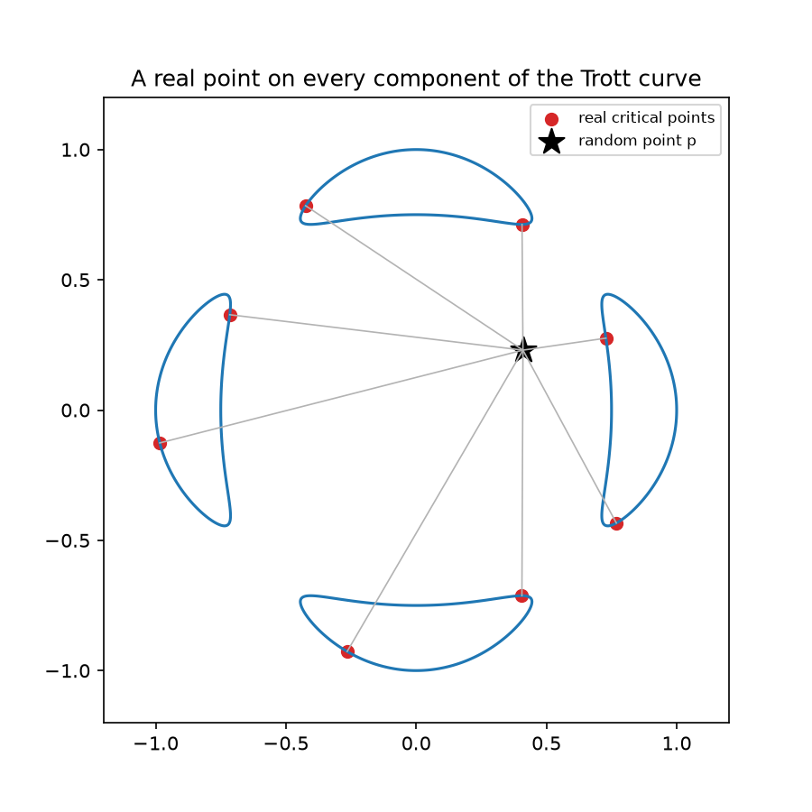
../../../_images/real_points.png — The four ovals of the Trott curve, the hardcoded random point \(p\) (★), the eight real distance-critical points (●), and a segment from \(p\) to each.¶

The method needs nothing special of the curve: pick a random real \(p\) (a generic choice avoids the measure-zero set where a component’s nearest point is non-isolated), build the same two equations for your \(f\), solve, and keep the real solutions.

Complete example¶

The whole tutorial as one runnable script – it saves the figure(s) shown above:

real_points.py¶

"""A real point on every component of the Trott curve.

Assembles the code fragments from the ``real_points`` tutorial into one
runnable program.  We build the critical-point (squared-distance) system for
the Trott quartic, solve it, keep the real solutions -- one real point on every
component -- and plot the curve, the random point p, and the distances.

Run:  python real_points.py
"""

import os
import matplotlib
matplotlib.use('Agg')            # headless backend, must precede pyplot import
import matplotlib.pyplot as plt

import numpy as np
from fractions import Fraction
import bertini

_OUT = os.path.dirname(os.path.abspath(__file__))


def build_system():
    """Build the square critical-point system for the Trott curve."""
    x, y = bertini.Variable('x'), bertini.Variable('y')
    f = 144*(x**4 + y**4) - 225*(x**2 + y**2) + 350*x**2*y**2 + 81

    # bertini differentiates the curve symbolically -- no hand-coded gradients
    fx, fy = f.differentiate(x), f.differentiate(y)

    # a hardcoded "random" real point p, with exact rational coordinates
    PX, PY = Fraction(41, 100), Fraction(23, 100)
    parallel = (x - bertini.coefficient(PX))*fy - (y - bertini.coefficient(PY))*fx

    crit_system = bertini.System()
    crit_system.add_variable_group(bertini.VariableGroup([x, y]))
    crit_system.add_function(f)
    crit_system.add_function(parallel)

    return crit_system, PX, PY


def solve_system(crit_system):
    """Solve and keep the real critical points -- the solver decides 'real'."""
    solver = bertini.ZeroDimSolver(crit_system, mptype='adaptive')
    solver.solve()

    crit = [(complex(s[0]).real, complex(s[1]).real)
            for s in solver.real_solutions()]      # the solver decides what "real" means

    assert len(crit) == 8                  # two per oval (nearest + farthest), all four ovals hit

    return crit


def plot(crit, PX, PY):
    """Plot the curve, the point p, the critical points, and the distances."""
    px, py = float(PX), float(PY)
    gx, gy = np.meshgrid(np.linspace(-1.2, 1.2, 500), np.linspace(-1.2, 1.2, 500))
    F = 144*(gx**4 + gy**4) - 225*(gx**2 + gy**2) + 350*gx**2*gy**2 + 81

    fig, ax = plt.subplots(figsize=(6, 6))
    ax.contour(gx, gy, F, levels=[0], colors='C0')          # the Trott curve
    for (cx, cy) in crit:
        ax.plot([px, cx], [py, cy], color='0.7', lw=0.8)    # distance to each critical point
    ax.scatter([c[0] for c in crit], [c[1] for c in crit], c='C3', s=40, label='real critical points')
    ax.scatter([px], [py], c='k', marker='*', s=200, label='random point p')
    ax.set_aspect('equal'); ax.legend(loc='upper right', fontsize=8)
    ax.set_title('A real point on every component of the Trott curve')

    fig.savefig(os.path.join(_OUT, 'real_points.png'), dpi=150)


def main():
    crit_system, PX, PY = build_system()
    crit = solve_system(crit_system)
    plot(crit, PX, PY)


if __name__ == '__main__':
    main()